Quick DS Reference
| Data Structure | Search | Insert | Delete | Notes |
|---|---|---|---|---|
| Linked List | O(n) | O(1)* | O(1)* | Fast insert/delete if node reference is known; no random access |
| Array | O(n) | O(n) | O(n) | O(1) index access but requires shifting on insert/delete |
| Hash Table | O(1) avg / O(n) worst | O(1) avg / O(n) worst | O(1) avg / O(n) worst | Depends on hash quality and collision handling |
| BST | O(log n) avg / O(n) worst | O(log n) avg / O(n) worst | O(log n) avg / O(n) worst | Can become skewed (degenerates into linked list) |
| AVL Tree | O(log n) | O(log n) | O(log n) | Strictly balanced → faster lookup |
| Red-Black Tree | O(log n) | O(log n) | O(log n) | Less strict balance → faster insert/delete than AVL |
| B-Tree | O(log n) | O(log n) | O(log n) | Optimized for disk/database systems (low I/O) |
| Heap (Binary Heap) | O(n) | O(log n) | O(log n) | Efficient for min/max only, not full search |
| Treap | O(log n) avg / O(n) worst | O(log n) avg / O(n) worst | O(log n) avg / O(n) worst | Randomized balancing (BST + heap property) |
- Linked List: efficient for head/tail access and fast insertion/deletion.
- Array: O(1) access to any element, good for indexed data.
- HashTable: O(1) expected access, but memory heavy and sensitive to collisions.
- Set: stores unique elements with fast lookup.
- Min/Max-Heap: priority queue structure for efficient min/max retrieval.
- Treap: BST + heap combination providing balanced search, insert, delete (O(log n) average).
- Graph: represents nodes and edges for networked relationships.
- BST (Binary Search Tree): simple sorted tree with O(log n) average operations.
- B-tree: balanced tree optimized for disk/database storage.
Big O
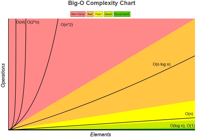
(fastest) 1 | log n | n | n log n | n^2 | 2^n | n! (slowest)O(log n): is when the the loop continuously divide the data/iteration
Basic Data Structures
- Record: DS with subitems called fields
- Similar to Java object, but no methods
- Array: ordered, indexed, mutable, allow dupes, homogenous (same type of items throughout), but need to be resized
- fast read, but slow insert
- Linked List same as array, but not indexed, and traversal is in one direction, unless it's a doubly linked list
- fast insert, but slow read
- Binary Trees: each node only have at most 2 children
- root: top node
- leaf: node w/o children
- Hash Table: unordered, each item is a bucket, key is obtaine by hashing/modding (%) the item
- fast lookup, but have big memory usage
- Heap: binary tree but have a priority with root being the highest priority
- max-heap: higher number has higher priority
- min-heap: lower number has higher priority
- Graph: DS to represent connections among items
Abstract Data Structures
class ADS
    Node head, tail;
    public insert(item) {}
    private insert(node) {}
    public remove(item) {}
private remove(node) {}- List: ordered collection of elements
- Implemented with: Array, Linked List
- Dynamic Array: array without fixed size (resizable)
- Implemented with: Array
- Stack: LIFO (Last In, First Out)
- Implemented with: Linked List (or Array)
- Queue: FIFO (First In, First Out)
- Implemented with: Linked List (or Array)
- Deque: Double-ended queue (insert/remove from both ends)
- Implemented with: Linked List
- Bag: unordered collection, allows duplicates
- Implemented with: Array, Linked List
- Set: unordered collection, no duplicates
- Implemented with: Binary Search Tree, Hash Table
- Priority Queue: elements processed based on priority
- Implemented with: Heap
- Map / Dictionary: key-value pair storage
- Implemented with: Hash Table, Binary Search Tree
Linked List
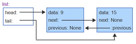
// Node Structure
class Node {
  data;
  Node next;
  Node prev;
}

class LinkedList {
  Node head, tail;

  public insert(item) {}
  public remove(item) {}
  public search(item) {}
}- Edge Cases:
- Check head == null for empty list (dummy node can simplify this)
- Updating head / tail when inserting or deleting
- Handle:
- Appending (tail changes)
- Prepending (head changes)
- Deleting head
- Deleting tail
- Operations Complexity:
- Search:
- Average / Worst: O(n)
- Insert / Delete:
- Average / Worst: O(1) (at head or tail node)
Hash Table
// Bucket Structure: the storage unit within a hash table
class Bucket {
  key;
  value;
  status; // EMPTY_SINCE_START | EMPTY_AFTER_REMOVAL | OCCUPIED
}

class HashTable {
  Bucket[] table;

  public insert(key, value) {}
  public remove(key) {}
  public search(key) {}
  private hash(key) {}
}- Collision Handling:
- Linear Probing
- Quadratic Probing
- Double Hashing
- Bucket Structure:
- key
- value
- isEmpty / status:
- EMPTY_SINCE_START
- EMPTY_AFTER_REMOVAL
- OCCUPIED
- After removal → mark as EMPTY_AFTER_REMOVAL (not fully empty)
- Search ends when:
- Key is found
- OR EMPTY_SINCE_START is encountered
- Hashing Concepts:
- Load Factor: (# of items) / (total buckets)
- Resize when threshold exceeded (e.g., 0.5)
- Hash Functions:
- Modulo (%)
- Mid-square (base 2)
- Multiplicative (for strings)
- Operations Complexity:
- Search / Insert / Delete:
- Average: O(1)
- Worst: O(n)
- Note: Worst case caused by collisions and depend on a good hash function to reduce collision rate
- Tradeoff: Large memory usage
Set
// Abstract Set
class Set {
  public union(setB) {}
  public intersection(setB) {}
  public difference(setB) {}

  public filter(condition) {}
  public map(func) {}
}- Properties:
- Unordered
- No duplicates
- Core Concepts:
- Cardinality: size of the set
- Two sets are equal if they contain the same elements (order does not matter)
- Set Operations:
- Union: X ∪ Y → elements in X or Y
- Intersection: X ∩ Y → elements in both X and Y
- Difference: X − Y → elements in X but not in Y
- Functional Operations:
- Filter: subset of X that satisfies a condition
- Map: new set with function applied to each element
- Operations Complexity:
- Search / Insert / Delete:
- Average / Worst: depends on implementation
- Typically:
- Hash Table → Avg: O(1), Worst: O(n)
- Balanced BST → Avg/Worst: O(log n)
Union-Find (Disjoint Set)
class UnionFind {
  int[] parent;
  int[] rank;

  public UnionFind(int n) {
    parent = new int[n];
    rank = new int[n];
    for (int i = 0; i < n; i++) parent[i] = i;
  }

  public int find(int x) {
    if (parent[x] != x) parent[x] = find(parent[x]); // path compression
    return parent[x];
  }

  public void union(int x, int y) {
    int rootX = find(x);
    int rootY = find(y);
    if (rootX == rootY) return;

    // union by rank
    if (rank[rootX] < rank[rootY]) {
      parent[rootX] = rootY;
    } else if (rank[rootX] > rank[rootY]) {
      parent[rootY] = rootX;
    } else {
      parent[rootY] = rootX;
      rank[rootX]++;
    }
  }

  public boolean connected(int x, int y) {
    return find(x) == find(y);
  }
}
Union-Find tracks a collection of elements partitioned into disjoint sets. It's used to see if two elements belong to the same group/set.It can only be used to tell if the nodes are connected directly/indirectly, but not whether Node A and B has a connected edge.
- Basic Terminology:
- Set: a group of connected elements
- Visually represented by a tree in Union-Find
- Representative / Root: the canonical element representing a set
- Parent: pointer to the next element toward the root
- Rank: an upper bound on the height of the tree representing a set
- Used to optimize union of two sets by attaching the shorter tree to the taller one
- Path compression: rewire every node when using
find(x)to point directly at the root
// Path compression
  public int find(int x) {
    if (parent[x] != x) parent[x] = find(parent[x]); // path compression
    return parent[x];
  }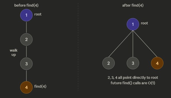
Path Compression
- find(x): returns the root of the set containing x
- union(x, y): merges sets containing x and y
- connected(x, y): checks if x and y are in the same set
- Path Compression: flattens the tree during find, making future finds faster
- Union by Rank / Size: attach smaller tree under larger to keep trees shallow
- Each operation: O(α(n)) ≈ nearly O(1), where α is the inverse Ackermann function
- Space: O(n) for parent and rank arrays
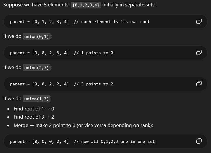
- We have a graph with nodes 0-4
- We do the following unions:
union(0,1),union(2,3), andunion(1,3) - Ending union-find will be
parent = [0, 0, 0, 2, 4] - From this union-find, we can tell nodes 0, 1, 2, 3 are connnected and node 4 is disconnected
- Can NOT tell if nodes 1 and 2 are directly connected
Binary Tree
class BinaryTree {
  Node root;

  public insert(item) {}
  public remove(item) {}
  public search(item) {}
}- Basic Terminology:
- Root: top node with no parent
- Leaf: node with no children
- Internal Node: node with at least one child
- Parent: node that has children
- Ancestors: all nodes from root → parent of a node
- Descendants: all nodes below a node
- Tree Metrics:
- Depth: # of edges from root → node (root = 0)
- Nodes with same depth form a level
- Height: # of edges from root → deepest node
- Types of Binary Trees:
- Full Binary Tree: every node has 0 or 2 children
- Complete Binary Tree: all levels are filled except possibly the last, filled left → right
- Perfect Binary Tree: all internal nodes have 2 children and all leaves are at same depth
- Operations Complexity:
- Search / Insert / Delete:
- Average: O(log n) (if balanced)
- Worst: O(n) (skewed tree)
Binary Search Tree (BST)
// Node Structure
class Node {
  key;
  Node left;
  Node right;
  Node parent;
}

class BST {
  Node root;
  public getHeight(node) {
    if node == null:
    return -1
    left_height = BST_get_height(node.left)
    right_height = BST_get_height(node.right)
    return 1 + max(left_height, right_height)
  }
}

// =============================================

// Traversals
// visit nodes in sorted order
inorder(node) {
  inorder(node.left)
  print(node)
  inorder(node.right)
}

// visit nodes in reverse sorted order
reverseInorder(node) {
  preorder(node.right)
  print(node)
  preorder(node.left)
}

// visit nodes in order of insertion
preorder(node) {
  print(node)
  preorder(node.left)
  preorder(node.right)
}

// visit all leaves first and root last
postorder(node) {
  postorder(node.left)
  postorder(node.right)
  print(node)
}- Properties:
- Left child ≤ parent
- Right child ≥ parent
- Smallest → leftmost node
- Largest → rightmost node
- Core Concepts:
- Successor: next larger node (usually leftmost node in right subtree)
- Predecessor: next smaller node (usually rightmost node in left subtree)
- Insertion:
- Start at root
- Traverse tree based on node value and insert as new leaf
- Removal:
- Find target node
- Find successor node
- Replace target with successor
- Traversals:
- Inorder: left → node → right (sorted order)
- Preorder: node → left → right (same as insertion order)
- Postorder: left → right → node (all leaves first and root last)
- Reverse Inorder: right → node → left (descending order)
- Operations Complexity:
- Search / Insert / Delete:
- Average: O(log n)
- Worst: O(n) (unbalanced tree)
Balanced BST
BST operations get worse the taller the tree gets so self-balancing trees are used to optimize the tree height
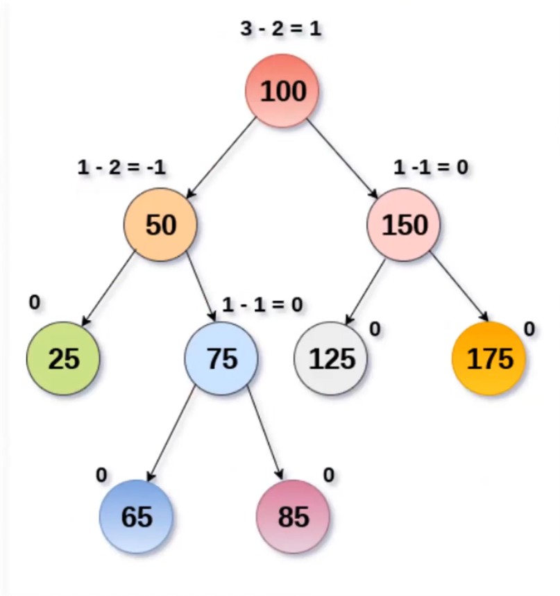
AVL Tree
A self-balancing BST that maintains balance by keeping track of a balance facotr on each node.
// Node Structure
class Node {
  key;
  Node left;
  Node right;
  Node parent;
  int height;
}- Self-balancing Binary Search Tree
- Each node must maintain a balance factor
- Balance Factor: height of left subtree − height of right subtree
- Balanced if balance factor is between -1 and 1
- Left heavy → balance factor > 0
- Right heavy → balance factor < 0
- Left Rotation at a node: RIGHT child becomes parent, move node down-left
- Right Rotation at a node: LEFT child becomes parent, move node down-right
- If left heavy → perform right rotation
- If right heavy → perform left rotation
- Double rotations:
- Left-Right (LR)
- Right-Left (RL)
- Insert: rebalance from inserted node → up to root by rotating based on balance factor
- Delete: rebalance from modified node → up to root by rotating based on balance factor
- Search / Insert / Delete:
- Average / Worst: O(log n)
- Note: stricter balance → faster lookup but more rotations than Red-Black Tree during insertion/deletion
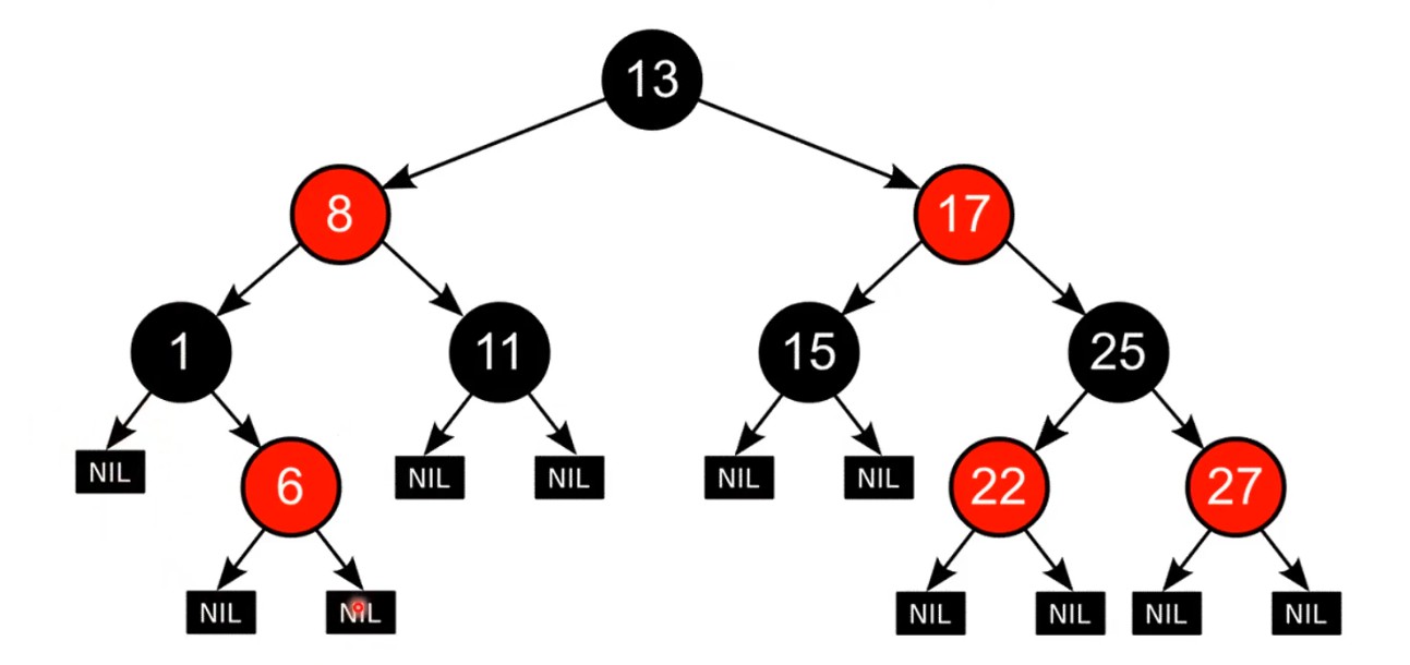
Red-Black Tree
A self-balancing binary search tree that maintains balance using recoloring.
Tree Rules
- Each node has a color: red or black
- Root and NIL (null leaves) are always black
- No two consecutive red nodes (a red node cannot have a red child)
- Every path from a node to its NIL descendants has the same number of black nodes (black height)
- Newly inserted nodes are always red
Tree Properties
- Shortest path = all black nodes
- Longest path = alternating red and black
- Longest path ≤ 2 × shortest path
- Balanced structure alternates: black → red → black → ...
Rotations
- Left Rotation at a node: RIGHT child becomes parent, move node down-left
- Right Rotation at a node: LEFT child becomes parent, move node down-right
- If left heavy → perform right rotation
- If right heavy → perform left rotation
Insertion Cases
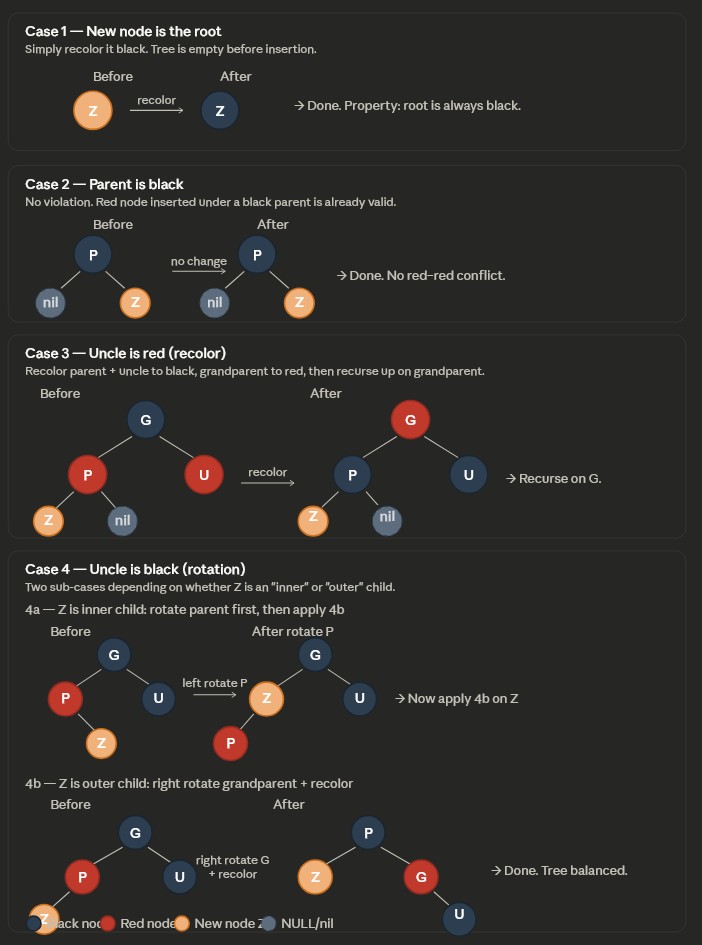
- Case 1: New node is root → recolor to black;
- Case 2: Parent is black → no fix needed;
- Case 3: Uncle is red → recolor parent & uncle to black, grandparent to red, then repeat upward
- Case 4: Uncle is black:
- 4a (zig-zag): Rotate at parent to make it linear
- 4b (linear): Rotate at grandparent and swap colors
Deletion Cases
- Case 1: Deleted node is red or root → no fix needed
- Case 2: Sibling is red → recolor and rotate at parent
- Case 3: Parent black, sibling and its children black → recolor sibling red, propagate up
- Case 4: Parent red, sibling and its children black → swap colors of parent and sibling
- Case 5: Sibling has one red child (inner case) → rotate at sibling to convert to Case 6
- Case 6: Sibling has outer red child → rotate at parent and fix colors
Operations Complexity
- Search / Insert / Delete:
- Average / Worst: O(log n)
- Compared to AVL trees:
- Looser balance
- Faster inserts/deletes
- Slightly slower lookups
Trie (Prefix Tree)
Non-binary tree to represent a set of strings
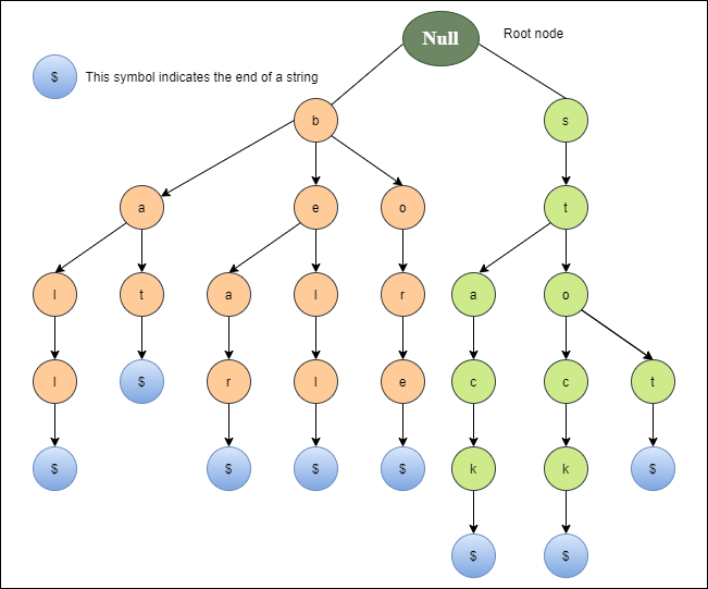
- Properties:
- Each path from root → node represents a prefix
- Terminal nodes mark the end of a valid word
- Without terminal nodes, tree wouldn't know if it has words like CAT or CATS
- Use Cases:
- Autocomplete
- Predictive text input
- Dictionary / spell checking
- Prefix-based searching
- Core Concepts:
- Search is based on prefix traversal, not full comparison
- Efficient for querying after typing a few characters
- No need to scan all results like a normal string search
- Removal:
- Unmark terminal node
- Delete nodes bottom-up if they have no children
- Stop when reaching a node that:
- Has other children, or
- Is the end of another word
- Operations Complexity:
- Search / Insert / Delete:
- Average: O(k)
- Worst: O(k)
- k = length of the word
- Note: time complexity is independent of number of stored words
B-Tree
Non-binary tree with K children and K-1 sorted, distinct keys; useful for lowering I/O operations or storing data in disk. Simiar to BST except B-trees are not restricted to having only one key and 2 children
// Node Structure
class BTreeNode {
  int keyCount;
  array keys[key0, key1];                    // sorted keys
  array children[child0, child1, child2];    // size = keyCount + 1
}- Non-binary tree with up to K children and K-1 sorted keys
- Keys inside a node are always sorted
- Each key partitions children into ranges (left < key < right)
- all keys of left subtree are less than that key
- all keys of right subtree are greater that key
key0 > child0's keyskey1 > child1's keys > key0- All leaf nodes are at the same level (balanced)
- Internal node with N keys has N+1 children
- Order (K) : max number of children per node
- Minimum keys per node: ceil(K/2) - 1
- Minimum does not apply to root node
- Maximum keys per node: K - 1
- B-Trees store multiple keys per node (unlike BST)
- Reduced tree height compared to BST
- Fewer node accesses → optimized for disk I/O
- 2-3-4 Tree is a B-Tree with order 4
- Databases (SQL indexing)
- File systems
- Large datasets stored on disk
- Minimizing disk reads/writes
- find the node with the key and return the whole node if it does, else recursively dig children nodes
Insert into correct leaf node and watch for overflow
- If node overflows past the max # of keys per node:
- Split node at median key
- Promote median key to parent
- Repeat upward if parent overflows
- If root overflows → create new root (height increases)
Delete key, make sure left subtree keys < internal node key < right subtree keys, and watch for underflow
- Case 1: targeted node is a leaf node
- Case 1a — Leaf has more than the minimum number of keys:
- Simply delete the key. No structural fix needed.
- Case 1b — Leaf is at minimum capacity (would underflow after deletion):
- Cannot just delete — must look at siblings and attempt to borrow.
- See Fixing Underflow below.
- Case 1a — Leaf has more than the minimum number of keys:
- Case 2: targeted node is an internal or root node
- Cannot remove directly — internal nodes act as separators for child subtrees.
- Replace the key with either:
- In-order predecessor — largest key in the left subtree, or
- In-order successor — smallest key in the right subtree
- Then delete the predecessor/successor from the leaf where it lives.
- This reduces the problem back to a leaf deletion (Case 1).
- Fixing Underflow — after a deletion causes a node to fall below the minimum number of keys:
- Sub-case A — Borrow from a sibling (rotation):
- If a neighboring sibling has more than the minimum number of keys, rotate through the parent.
- Pull the parent's separator key down into the deficient node.
- Push the sibling's closest key up to replace it in the parent.
- Also called a left rotation or right rotation.
- Sub-case B — Merge with a sibling:
- If no sibling can spare a key, merge the deficient node with one sibling.
- Pull the parent's separator key down into the merged node.
- The parent loses a key — this may cause the parent to underflow too (cascades upward).
- Sub-case C — Cascade to the root:
- If merges propagate all the way up and the root ends up with 0 keys, the root is deleted.
- The tree shrinks by one level — the only way a B-tree's height decreases.
- Sub-case A — Borrow from a sibling (rotation):
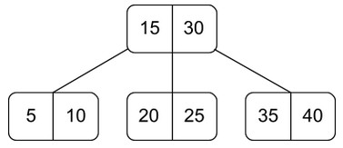
- Example:
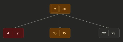
Part 1: Initial B-tree. 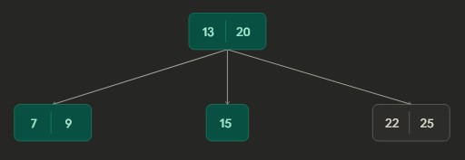
Part 2 - Borrowing: After deleting key 4; the node borrowed from its sibling. Rotated key 9 from parent and key 13 from sibling 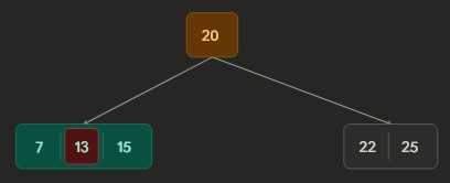
Part 3 - Merging: After deleting key 9; the node merge with sibling key 15 and parent key 13.
- Search / Insert / Delete:
- Average / Worst: O(log n)
- Lower height than BST → fewer node accesses
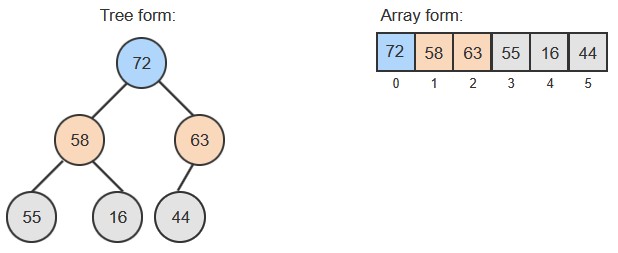
Heap (Binary Heap)
Heaps are priority queue and are normally shown visually as a tree, but it's implemented as an array
// Structure (Array-based)
class Heap {
  array data[];
  int size;
}

// Index mapping for a node at index i:
parent index = floor((i - 1) / 2)
leftChild index = 2i + 1
rightChild index = 2i + 2- Properties:
- Mapping for a node at index i:
parent index = floor((i - 1) / 2)leftChild index = 2i + 1rightChild index = 2i + 2- Complete binary tree (last level filled left → right)
- Max-Heap: parent ≥ children
- Min-Heap: parent ≤ children
- Not fully sorted (only guarantees parent-child ordering)
- Core Concepts:
- Percolate Up: move node up until heap property is satisfied
- Percolate Down: move node down by swapping with larger/smaller child
- Heapify: convert unordered array into a valid heap
- Heapsort: repeatedly remove root to produce sorted array
- Heapify Process: turning an unsorted array of size n into a heap array
- Start at last non-leaf node:
floor(n/2) - 1 - Apply percolate down
- Repeat upward until reaching root
- Builds heap in O(n) time
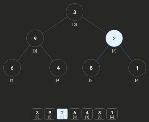
Heapify Max-Heap Part 1: start at last non-leaf node and percolate down 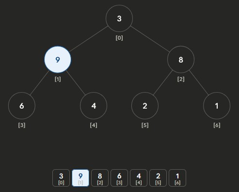
Heapify Max-Heap Part 2: repeat for next non-leaf node 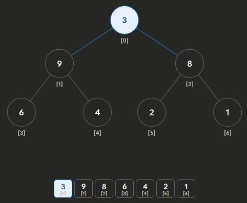
Heapify Max-Heap Part 3: keep going until root 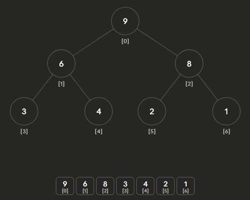
Heapify Max-Heap Part 4: finalized heap - Start at last non-leaf node:
- Insertion:
- Insert at last position (end of array)
- Percolate up to restore heap property
- Removal:
- Remove root (highest/lowest priority)
- Replace with last element
- Percolate down to restore heap property
- Operations Complexity:
- Search:
- Average/Worst: O(n)
- Min/Max lookup: O(1)
- Insert / Delete:
- Average: O(log n)
- Worst: O(log n)
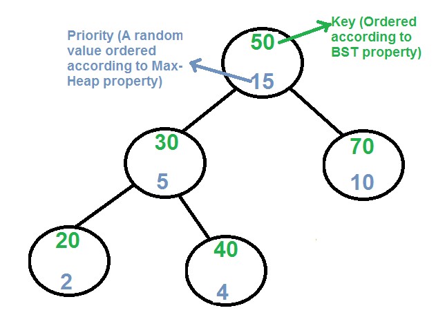
Treap (BST + Heap)
// Node Structure
class TreapNode {
  key;
  priority;
  TreapNode left;
  TreapNode right;
  TreapNode parent;
}- Properties:
- Combination of Binary Search Tree and Max-Heap and satisfies both DS properties
- Each node has a key and a random priority
- BST property: leftChild key < parent key < rightChild key
- Heap property: parent priority > children priorities
- Core Concepts:
- Tree stays probabilistically balanced due to random priorities
- No strict rebalancing rules like AVL or Red-Black trees
- Rotations maintain heap property (instead of swaps like heaps)
- Search:
- Same as BST (compare keys and traverse left/right)
- Insertion:
- Insert node using BST rules
- Assign random priority to the inserted node
- Percolate up based on priorities using rotations:
- If you want left child to replace parent → rotate right at parent
- If you want right child to replace parent → rotate left at parent
- Deletion:
- Set node priority to −∞ (lowest)
- Percolate down using rotations until node becomes a leaf
- Remove the node
- Operations Complexity:
- Search / Insert / Delete:
- Average: O(log n)
- Worst: O(n) (extremely unlikely due to randomness)
Graph
// Node / Edge Structure
class Node {
  key;
}
class Edge {
  fromNode;
  toNode;
  weight;
}

// Graph Structure w/ Adjacency List
class Graph {
  map<Node, list<Node>> adjacencyList;

  addNode(node) {}
  addDirectedEdge(u, v) {}
  addUndirectedEdge(u, v) {}
}- Properties:
- Collection of nodes (vertices) and edges
- Can be cyclic or acyclic
- Trees are acyclic graph
- Can be directed or undirected
- Edges may have weights (cost, time, distance)
- Core Concepts:
- Path: sequence of edges from one node to another
- Distance: number of edges in the shortest path
- Adjacency: nodes directly connected by an edge
- Directed Edge: one-way connection
- Undirected Edge: two-way connection
- Graph Representations:
- Adjacency List:
- Each node stores a list of its neighbors
- Space: O(V + E)
- Adjacency Lookup: O(V) worst case (usually small in practice)
- Most commonly used (efficient for sparse graphs)
- Adjacency Matrix:
- 2D matrix where rows/columns represent nodes
- 1 = edge exists, 0 = no edge
- Diagonal (node to itself) = 0
- Space: O(V²)
- Adjacency Lookup: O(1)
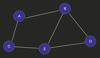
Undirected Graph 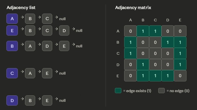
Different ways to store a graph. - Adjacency List:
- Special Cases:
- Tree: an acyclic graph
- Weighted Graph: edges have cost/distance/time values
- Negative Weight Cycle:
- No shortest path exists
- Path cost can decrease indefinitely
- Use Cases:
- Maps and navigation (shortest path)
- Social networks (connections between users)
- Recommendation systems
- Operations Complexity:
- Add Node: O(1)
- Add Edge: O(1)
- Space:
- Adjacency List: O(V + E)
- Adjacency Matrix: O(V²)
Graph Traversal Techniques (BFS & DFS)
Breadth-First Search (BFS):
- Visits nodes level by level
- Uses a queue (FIFO)
- Explores all neighbors before going deeper
- Best for shortest path (unweighted graphs)
- Steps
- Add starting node to queue
- Pop the queue and add all neighbors into
queueandvisitedSetif not already invisitedSet - Process current node
- Pop from queue again and repeat until queue is empty
// Breadth-First Search (BFS)
bfs(start) {
  queue = new Queue()
  visited = new Set()

  queue.enqueue(start)
  visited.add(start)

  while queue is not empty:
    node = queue.dequeue()
    for neighbor in node.neighbors:
      if neighbor not in visited:
        queue.enqueue(neighbor)
        visited.add(neighbor)

    process(node)
}
Depth-First Search (DFS):
- Explores deepest path first
- Uses a stack (LIFO) or recursion and the internal program stack
- Backtracks after reaching a dead end
- Good for exploring all paths and cycle detection
- Steps
- Dig starting node recursively or add starting node to
stack - Pop
stackand process node if not invisitedSet - Add current node to
visitedSet - Dig neighbors recursely or add neighbors into
stackif not invisitedSet - Do until
stackis empty
// Depth-First Search (DFS - Recursive)
dfsRecursive(node, visited) {
  if node in visited:
    return

  process(node)
  visited.add(node)

  for neighbor in node.neighbors:
    dfsRecursive(neighbor, visited)
}
Core Concepts:
Handling Cyclic / Acyclic:- Visited Set: prevents revisiting nodes
- Required for:
- Cyclic graphs
- Undirected graphs
- Not strictly required for trees (acyclic)
- BFS: queue → level-order traversal (visit all nodes in same level first)
- DFS: stack/recursion → depth traversal (visit a whole branch first)
- BFS finds shortest path (unweighted), DFS does not guarantee it
- Add node to
visitedwhen:- BFS → when enqueueing the node
- DFS → when pushing the node to stack or processing the node
- Avoid adding nodes already in visited set
- BFS / DFS:
- Time: O(V + E)
- Space: O(V)