Quick Algorithms Refence
| Algorithm | Best Case | Average Case | Worst Case | Notes / Stability |
|---|---|---|---|---|
| Bubble Sort | O(n) | O(n²) | O(n²) | Stable, simple |
| Selection Sort | O(n²) | O(n²) | O(n²) | Not stable (unless modified) |
| Insertion Sort | O(n) | O(n²) | O(n²) | Stable, efficient for small / nearly sorted arrays |
| Merge Sort | O(n log n) | O(n log n) | O(n log n) | Stable, requires extra space |
| Quick Sort | O(n log n) | O(n log n) | O(n²) | Not stable, in-place; pivot choice matters |
| Quickselect | O(n) | O(n) | O(n²) | In-place selection of k-th element; pivot choice matters |
| Radix Sort | O(nk) | O(nk) | O(nk) | Stable, non-comparison sort; k = number of digits |
- DFS (Depth-First Search): explores graph nodes deeply/per branch before backtracking.
- BFS (Breadth-First Search): explores graph nodes level by level.
- Merge Sort: divide-and-conquer sort with O(n log n) performance.
- QuickSelect: finds k-th smallest element efficiently using partitioning.
- Radix Sort: non-comparison integer sort using digit-based bucket passes.
- Bucket Sort: distributes elements into value-range buckets, then sorts each.
- Topological Sort: creates subtree (DAG) based on prerequisites / ordering of nodes edges.
- Shortest Path Algorithms: algorithms to find the shortest path to EACH node from a starting node in a graph.
Recursion
// Example: Binary Search (Recursive)
// Break the problem into smaller problems and work on those
binarySearch(arr, left, right, target) {
  if left > right:
    return -1

  mid = (left + right) / 2

  if arr[mid] == target:
    return mid
  else if target < arr[mid]:
    return binarySearch(arr, left, mid - 1, target)
  else:
    return binarySearch(arr, mid + 1, right, target)
}- Definition:
- A function that calls itself to solve smaller subproblems
- Stops when reaching a base case(s)
- Core Components:
- Base Case(s): stopping condition(s)
- Recursive Case: reduces problem size
- Number of base cases = number of required initial conditions
// Example: Fibonacci requires 2 base cases because it needs 2 initial conditions fibonacci(n) { if n == 0: return 0 if n == 1: return 1 return fibonacci(n - 1) + fibonacci(n - 2) } - Visualization:
- Recursive calls form a call tree
- Each node represents a function call
- Leaves represent base cases
- Time Complexity Analysis:
- General form: T(n) = work per call + recursive calls
- Example:
- Binary Search → T(n) = O(1) + T(n/2)
- Time Complexity → O(log n)
- Key idea:
- How much the problem size shrinks each call
- How many recursive calls are made
- Common Patterns:
- Linear Recursion:
- T(n) = T(n-1) + O(1) → O(n)
- Divide & Conquer:
- T(n) = T(n/2) + O(1) → O(log n)
- Branching Recursion:
- T(n) = 2T(n-1) + O(1) → O(2ⁿ)
- Example: Fibonacci (naive)
- Linear Recursion:
- Space Complexity:
- Depends on recursion depth (call stack)
- Examples:
- Binary Search → O(log n)
- Linear recursion → O(n)
- Key Insights:
- Recursion ≈ implicit stack (function call stack)
- Can often be converted to iteration using a stack
- Performance depends on:
- Number of calls
- Work per call
Algorithmic Paradigms
Algorithmic paradigms are general strategies or approaches for designing algorithms—basically, ways of thinking about how to solve problems.
- Heuristic:
- Rule-of-thumb or approximation strategy
- Trades optimality for speed/practicality
- Common in large or complex problem spaces
- Divide and Conquer:
- Break problem into smaller independent subproblems
- Solve recursively
- Combine results
- Examples: Merge Sort, Binary Search
- Greedy:
- Make the locally optimal choice at each step
- Like picking highest priority or the lowest weight for the next step
- Does not reconsider previous decisions
- Works only when local optimum leads to global optimum
- Examples: Dijkstra (no negative weights), Activity Selection
- Relaxation:
- Repeatedly improve a solution estimate
- Common in shortest path algorithms
- Example idea:
- If a shorter path to a node is found → update it
- Used in: Dijkstra, Bellman-Ford
- Dynamic Programming:
- Break problem into overlapping subproblems
- Store and reuse previous results (memoization/tabulation)
- Avoids redundant computation
- Two approaches:
- Top-down (memoization)
- Bottom-up (tabulation)
- Key Differences:
- Divide & Conquer: independent subproblems
- Dynamic Programming: overlapping subproblems
- Greedy: no backtracking, local decisions only
- Heuristic: approximate, not guaranteed optimal
Graph Pathfinding Algorithms
Goal: find shortest path from a starting node to EACH node in the graph
When selecting algorithm, it's important to watch for existant of negative edge weight and negative weight cycle in graph
Dijkstra’s Algorithm
- Goal: find shortest path from a starting node to EACH node in the graph
- Limitation: can not be used if there is a negative edge weight in the graph
- Uses greedy + relaxation
- Processes nodes in order of smallest distance (min heap)
- Data Structures:
PathTracker: maps each node to its total distance from A and its previous node on the path from AminHeap: priority queue of total distance to reach the node starting from node A- Use Cases:
- Network routing / navigation systems
- Operation Complexity:
- Time complexity: O(E log V) (with min heap)
- V = number of vertices/nodes
- E = number of edges
- Steps:
- Use
min-heapand prioritize the closest node to walk through graph - Use another DS,
PathTracker, to keep track of "Distance from A" and "Previous Node" for each node in graph - Every time neighbor nodes are added to nodeStack, update the
PathTrackerwith the total distance from A and previous node IF the NEW total distance from A is less than CURRENT total distance from A insidePathTracker - At the end,
PathTrackerwill have the shortest path from A to any node in the graph - Example:
- Push starting node into
minHeap - Starting
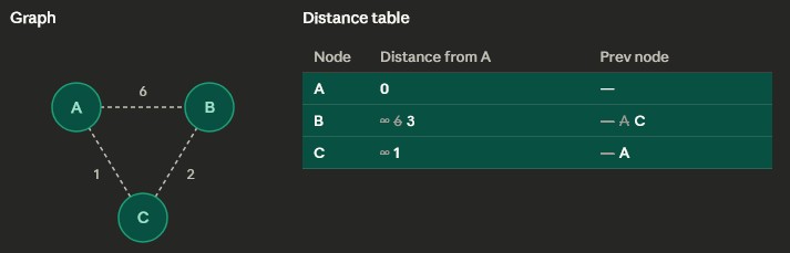
minHeap: [ (0, A) ] = (total distance from A, corresponding node) - Pop
minHeapand visit A: A is the starting node with distance 0, so it's processed first. Both B and C get their first real distances — 6 and 1 respectively — crossed over from ∞. - Push 2 new total distance and nodes to
minHeap minHeapafter visiting A: [ (1, C), (6, B) ]- Pop
minHeapand visit C: C wins the next pick with the smallest tentative distance (1). From C, we can reach B at cost 1+2 = 3, which beats B's current value of 6. So 6 gets crossed out and replaced with 3. - Push the new total distance to node B into
minHeap minHeapafter visiting C: [ (3, B), (6, B) ]- Pop
minHeapand visit B: B is processed last with its final distance of 3. C is already visited, so nothing changes. minHeapafter visiting B: [ (6, B) ]- Pop
minHeap, but the total distance is bigger than what's inPathTrackerso it's ignored.minHeap is empty so algorithm is done. - Pseudocode:
PathTracker table with starting node A// Dijkstra's Algorithm (Min Heap)
dijkstra(graph, startNode) {
// PathTracker is split into two maps
totalDist = map(default = infinity)
prevNode = map()
minHeap = new MinHeap()
totalDist[startNode] = 0
minHeap.insert((0, startNode))
while minHeap not empty:
(currDist, node) = minHeap.extractMin()
for neighbor in graph[node]:
newDist = currDist + weight(node, neighbor)
if newDist < totalDist[neighbor]:
totalDist[neighbor] = newDist
prevNode[neighbor] = node
minHeap.insert((newDist, neighbor))
}Bellman-Ford Algorithm
- Goal: find shortest path from a starting node to EACH node in the graph
- Limitation:
- Work with negative edge weight, but can not be used if there is a negative weight CYCLE in the graph
- Algorithm will detect negative cycle though
- Data Structures:
PathTracker: maps each node to its total distance from A and its previous node on the path from AedgeList: queue of all lists algorithm will go through for each iteration- Uses relaxation
- Perform V-1 iterations + 1 more as a negative-cycle check - V = number of vertices/nodes
- In the last iteration, if distance in
PathTrackertable improves → cycle exists - Bellman-Ford does not walk through a graph like Dijkstra, but loop through every edge in the
edgeListand update thePathTrackertable the same way as Dijkstra - Use Cases:
- Path finding with negative edge weight
- Operation Complexity:
- Time complexity: O(V × E)
- V = number of vertices/nodes
- E = number of edges
- Steps:
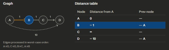
- 1st iteration: loop through every edge and if edge is connection to the starting point or has a PREVIOUSLY checked connection to starting point, calc weight and update
PathTrackertable - 2nd ... V-1 iterations: same thing as first, but the table gain more data on edges connected to starting point with each iteration
- Vth (Last iteration): negative-cycle check; if the shortest distance still changes in the
PathTracker, then there is a negative-cycle - Example: Starting node is A, and using the worst order for looping through edges
- Pseudocode:
PathTracker table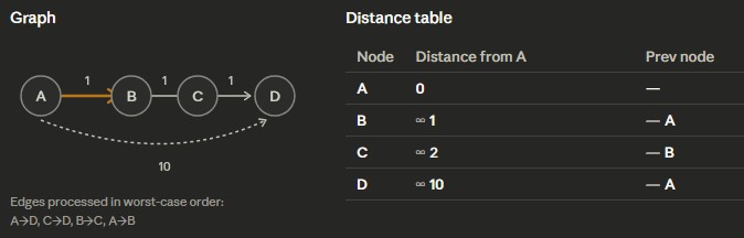
PathTracker accordingly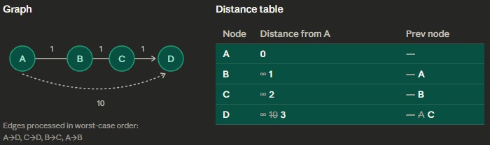
PathTracker table// Bellman-Ford Algorithm
bellmanFord(edges, V, start) {
// PathTracker is split into two maps
totalDist = map(default = infinity)
prevNode = map()
// Relax edges V-1 times
for i from 1 to V-1:
for (u, v, w) in edges:
if totalDist[u] + w < totalDist[v]:
totalDist[v] = totalDist[u] + w
prevNode[v] = u
// Negative cycle check
for (u, v, w) in edges:
if totalDist[u] + w < totalDist[v]:
return false // negative cycle exists
return totalDist
}Topological Sorts
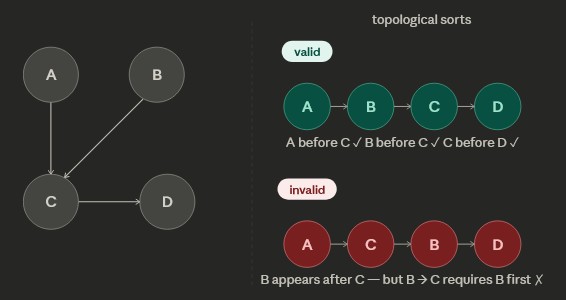
- Goal: create subtrees of the graph with the nodes ordered as a Directed Acyclic Graph (DAG)
- Data Structures:
resultStack: keep track of the current topological sortvisitedSet: keep track of visited nodes to avoid cycle- Ensures all edges go from earlier → later
- Uses DFS + postorder
- Use Cases:
- Use for task scheduling with prerequesites requirement
- Making a valid course/class sequence based on prerequesites
- Dependency resolution (making dependency 1 is installed before 2, etc)
- Operation Complexity:
- Time complexity: O(V + E)
- V = number of vertices/nodes
- E = number of edges
- Steps:
- Do DFS on the starting node and every non-visited node of its children and the whole graph
- Push node to
resultStackafter visiting all its children (postorder) - Reverse the
resultStackto get one possible topological sort for the graph - Pseudocode:
// Topological Sort (DFS)
topoSort(graph) {
  for node in graph:
    if node not in visited:
      dfs(node)

  return reverse(resultStack)
}

dfs(node) {
  visited.add(node)

  for neighbor in graph[node]:
    if neighbor not in visited:
      dfs(neighbor)

  resultStack.push(node)         // postorder
}
Minimum Spanning Tree (MST)
Minimum spanning tree (MST) is a subtree of the graph with the minimum total edge weight (i.e. what's the cheapest way to connect all points together). MST only keeps cheapest edge for each vertex and avoid more expensive redundant edges.
- Goal: connect all vertices in a graph with the minimum total edge weight
- Requirements:
- Graph must be weighted
- Graph must be connected (no vertices are disconnected from rest)
- No cycles allowed (must remain a tree)
- Total edges in MST = V - 1
- Uses greedy strategy (pick cheapest valid edges)
Prim’s Algorithm
- Goal: build MST by expanding from a starting node
- Data Structures:
visitedSet: tracks nodes already in MSTminHeap: stores edges prioritized by weight → (weight, from, to)mst: list of edges in the final MST- Use Cases:
- Best for dense graphs (many edges)
- Operation Complexity:
- Time complexity: O(E log V)
- V = number of vertices
- E = number of edges
- Steps:
- Pick any node as the starting node
- Add all its edges into
minHeap - Pop the smallest edge from
minHeap - If the destination node is already visited → skip
- Otherwise:
- Add edge to MST
- Mark node as visited
- Push all outgoing edges of that node to unvisited nodes into
minHeap
- Repeat until MST has V - 1 edges
- Pseudocode:
// Prim's Algorithm
prim(graph, startNode) {

  visitedSet = new Set()
  minHeap = new MinHeap() // (weight, from, to)
  mst = []

  visitedSet.add(startNode)

  for edge in graph[startNode]:
    minHeap.insert(edge)

  while minHeap not empty:
    (weight, u, v) = minHeap.extractMin()

    if v in visitedSet:
      continue

    mst.add((u, v, weight))
    visitedSet.add(v)

    for edge in graph[v]:
      if edge.to not in visitedSet:
        minHeap.insert(edge)
}
Kruskal’s Algorithm
- Goal: build MST by selecting smallest edges globally
- Data Structures:
edgeList: all edges sorted by weightUnionFind: tracks connected componentsmst: list of edges in the final MST- Use Cases:
- Best for sparse graphs (few edges)
- Operation Complexity:
- Time complexity: O(E log E)
- V = number of vertices
- E = number of edges
- Steps:
- Sort all edges by weight (ascending)
- Initialize each node as its own set
- Iterate through sorted edges
- If edge connects two different sets:
- Add edge to MST
- Union the sets
- Stop when MST has V - 1 edges
- Pseudocode:
// Kruskal's Algorithm
kruskal(edges, V) {

  sort edges by weight
  uf = new UnionFind(V)
  mst = []

  for (u, v, w) in edges:
    if uf.find(u) != uf.find(v):
      mst.add((u, v, w))
      uf.union(u, v)

    if mst.size == V - 1:
      break
}
Sorting Algorithms
Bubble Sort:- Iterates through a list, swapping adjacent elements if the second is less than the first.
- 1st iteration places the largest element at the end; subsequent iterations place the next largest elements.
- Average/Worst Case: O(n²)
- Splits the array into imaginary sorted/unsorted partitions.
- Iterates through the unsorted part to find the lowest element, then swaps it with the current element.
- Example:
[2 5 8 1 10]→[(sorted) (unsorted)]→[(1) (5 8 2 10)] - Average/Worst Case: O(n²)
- Also splits array into sorted/unsorted partitions, but moves the unsorted element into the sorted region instead of finding the lowest first.
- Example:
[2 5 8 1 10]→[(sorted) (unsorted)]→[(2 5) (8 1 10)] - Average/Worst Case: O(n²)
- Best Case (already sorted): O(n)
Merge Sort:
- Divide and merge: recursively split the list in half until each sublist has 1 element, then merge while sorting.
- Merging: repeatedly pick the smaller element from the two sublists; if one sublist empties, append the other.
- Example:
[2 5 8 1 10]→[[2 5] [1 8] [10]]→[[1 2 5 8] [10]] - Average/Worst Case: O(n log n)
Quick Sort:
- Pick a pivot element; partition elements less than pivot to left, greater to right.
- Recursively apply to left and right partitions until each has 1 or 0 elements.
- Example:
[2 5 8 1 10]→[[2 5 1] 8 [10]]→[[2 1] 5 [] 8 [10]]→[[] 1 [2] 5 [] 8 [10]] - Average/Best Case: O(n log n)
- Worst Case: O(n²), depends on pivot choice
- Uses Quick Sort partitioning to find the k-th smallest element without sorting the whole list.
- Pivot index is used as reference: if k < pivot index → search left; if k > pivot index → search right; else pivot is answer.
- Note: if looking for k-th smallest, desired index = k-1 (2nd smallest → index 1)
- Average/Best Case: O(n)
- Worst Case: O(n²)
Radix Sort:
- Designed for arrays of integers.
- Divide elements into buckets by digit place (ones, tens, hundreds…); collect in order (FIFO) and repeat for next higher digit.
- Final list after highest digit pass is sorted.
- Average/Worst Case: O(nk), k = number of digits
- Simpler than Radix Sort.
- Buckets labeled as ranges; divide elements into buckets based on value, then sort each bucket.
- Average Case: O(n + k)
- Worst Case: O(n²)
Heapify / Heap Sort:: more details
- Heapify: transform array into a max-heap or min-heap (complete binary tree with heap property).
- Heap Sort: repeatedly extract root (max/min) and re-heapify remaining elements.
- Time Complexity: O(n log n) for heap sort, O(n) to build the heap.
Topological Sort:: more details
- Sort nodes of a DAG so that for every edge u → v, u comes before v.
- Implemented via DFS or Kahn’s algorithm (BFS with indegree tracking).
- Time Complexity: O(V + E), V = vertices, E = edges.